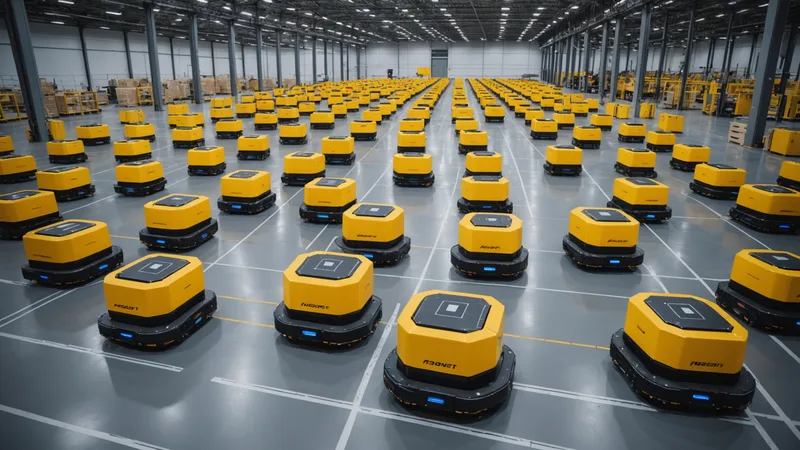
When 3PL operators first ask us about expected fleet utilization after deploying Botpylon, they often frame the question around their current numbers. "We are at 68% right now. Is that good?" The answer depends on what you are counting and how the fleet is being dispatched, but 68% in an uncoordinated mixed-fleet deployment is actually not far from the industry norm for uncoordinated operations. The question is not whether 68% is acceptable in absolute terms. The question is what is structurally preventing the fleet from doing better.
Robot fleet utilization is one of those metrics that sounds simple but carries several layers of definitional ambiguity. Getting the benchmark right requires being precise about what you are actually measuring.
Defining Robot Utilization Correctly
Fleet utilization is the fraction of available robot time that a robot spends doing productive work, where productive work means actively carrying a payload, executing a pick task, or traveling directly toward a task destination. Non-utilization time includes stop-and-wait states (robot has a task but cannot move due to congestion), idle states (no task assigned), charging (robot at a charging station), and fault/maintenance states.
The important distinction is between idle (no task available) and stop-and-wait (task assigned but movement blocked). These look similar in a simple utilization dashboard, but they have different causes and different solutions. Low idle time but high stop-and-wait time means the dispatch engine has task supply but is creating traffic conflicts. Low stop-and-wait but high idle time means task supply is the constraint, which is a WMS or workflow problem rather than an orchestration problem.
For utilization benchmarking purposes, productive utilization = (time with assigned task in motion) / (total available shift time). This excludes charging (which is necessary infrastructure, not waste), faults (which are maintenance issues), and properly planned idle time at shift transitions. Stop-and-wait time counts as non-utilization because the robot has a task and should be moving but is not.
What the Industry Baseline Actually Looks Like
Across multi-vendor deployment patterns observed in the fulfillment sector, productive utilization in uncoordinated or single-vendor-FMS-only environments tends to cluster in the 63-74% range during active picking periods. The variance within that range correlates primarily with fleet size relative to floor area, pick zone density, and whether the deployment uses any form of dynamic task batching.
The 65-72% range most commonly cited in industry practitioner discussions covers mid-size deployments of 40-150 AMRs on a single fulfillment floor. Very small fleets (under 25 robots) often achieve higher utilization because the coordination overhead is manageable with simpler dispatch and congestion events are rare. Very large fleets (200+ robots) can drop below 60% utilization in uncoordinated deployments because congestion events become frequent enough to create significant cascading stop-and-wait time.
Coordinated deployments with dynamic dispatch, congestion-aware routing, and cross-vendor fleet visibility consistently reach 88-94% productive utilization during mid-shift steady-state periods. The gap between uncoordinated and coordinated is largest during wave transitions (when new batches of tasks are released) and during peak load periods when floor density is highest.
Where the Missing 20-25% Goes
If an uncoordinated fleet at 68% productive utilization were to reach 90%, that 22-point gap represents roughly 2.6 additional productive hours per robot per 12-hour shift. For a 60-robot fleet, that is 156 robot-hours per shift of additional capacity. At a pick rate of 150 units per robot-hour, that translates to roughly 23,000 additional units of pick throughput per shift, without adding a single robot.
The gap breaks down into identifiable sources. Stop-and-wait congestion typically accounts for 8-12 percentage points of utilization loss in uncoordinated fleets. This is the clearest win from congestion-aware dispatch: robots spend less time waiting at aisle entries or behind other robots because the dispatch engine routes them away from congested zones before they arrive.
Suboptimal task assignment accounts for another 5-8 percentage points. Without fleet-wide task visibility, vendor FMS assigns tasks based on proximity within that vendor's robot pool, ignoring whether another robot (from a different vendor) is already closer to the target location or whether the assigned robot's route takes it through a congested zone. A unified dispatch layer that sees all robots assigns tasks to minimize total fleet travel time, not just per-robot travel time.
The remaining gap typically comes from charging schedule inefficiency (3-5 points) and wave transition dead time (2-4 points). Charging schedule optimization requires knowing the battery state of all robots across vendors and planning charge cycles that do not pull too many robots off the floor simultaneously. Wave transition dead time is the period between a completed pick wave and the release of the next wave's tasks, during which robots sit idle waiting for new assignments.
A Scenario: 85 AMRs, Two Floors, Mixed Vendors
A mid-size fulfillment operation in the Southwest was running 85 AMRs across two floors, with vendor FMS from two different suppliers managing each vendor's robots independently. Before coordinated dispatch, their measured productive utilization averaged 71% across full shifts, dropping to 64% during peak pick windows when floor density was highest.
The stop-and-wait analysis showed that most congestion events concentrated at the ramp access points between the two floors and at the four highest-velocity pick zones on floor one. These were predictable hotspots that both FMS systems were routing toward simultaneously without awareness of the other vendor's traffic.
After integrating a unified orchestration layer, the floor graph captured both vendors' robot positions and used that state for cross-vendor routing decisions. Ramp access scheduling was added as a gated resource, with the orchestration layer queuing ramp approach sequences rather than allowing simultaneous convergence. Within two weeks of steady-state operation with the unified dispatch, productive utilization settled at 91% during peak windows and 93% during mid-shift steady state. Stop-and-wait events dropped by 76%.
These numbers are from a specific deployment configuration and should not be assumed to transfer identically to different floor geometries or fleet sizes. The pattern, however, is consistent: unified visibility plus coordinated dispatch eliminates the cross-vendor blindspot that accounts for the majority of stop-and-wait time in mixed fleets.
Utilization Ceilings and Honest Limits
It is worth being direct about what utilization optimization cannot do. A fleet operating at 93% productive utilization is not at 100%, and reaching 100% would actually be a sign of system stress rather than peak performance. Robots need to charge. Maintenance windows are necessary. Brief idle periods at task transitions are normal operational states, not waste.
The practical ceiling for healthy productive utilization in a well-coordinated fulfillment floor is around 92-95% during active picking periods. Above that range, the fleet has insufficient slack to handle robot faults or priority order spikes without cascading delays. Operating closer to 90-92% leaves the system with enough flex capacity to absorb variability without degrading.
We are also not claiming that utilization improvement translates linearly into throughput improvement. At high utilization, throughput gains depend on whether the additional robot-hours are going to picks that feed the packing and shipping stages at a rate those stages can absorb. Optimizing robot utilization without addressing downstream throughput constraints (packing station capacity, sortation bandwidth) shifts the bottleneck rather than eliminating it. Fleet utilization benchmarks are one input to an operations assessment, not the whole picture.
How to Establish Your Own Baseline
Before evaluating any dispatch optimization solution, establish a clear baseline measurement. Pull robot telemetry logs for a representative two-week period (ideally including at least one peak volume week). Classify each robot state as productive (task in motion), stop-and-wait (task assigned, zero velocity for more than 15 seconds), idle (no task assigned), charging, or fault. Calculate the fraction of total available shift hours that falls into each category.
The ratio of stop-and-wait to idle tells you the primary optimization opportunity. High stop-and-wait means congestion management is the lever. High idle means task supply or dispatch logic is the constraint. Both are solvable, but with different tools. A floor with 15% stop-and-wait and 12% idle has more headroom from congestion-aware routing than a floor with 5% stop-and-wait and 22% idle, where the orchestration layer would deliver modest gains and the real fix is WMS-side wave management.